Flow Matching¶

Flow matching learns a time-conditioned velocity field \(v_\theta(x, t)\) that transports a simple source density (Gaussian noise at \(t=0\)) onto the data distribution (at \(t=1\)). It is simulation-free: no sampler runs inside the training loop, so training scales like ordinary supervised regression.

The objective¶

Given an interpolant that defines, for each \(t \in [0, 1]\), an intermediate point \(x_t\) and its conditional target velocity \(u_t\), the model is regressed onto \(u_t\):

\[ \mathcal{L}_\text{FM}(\theta) = \mathbb{E}_{t,\, x_0,\, x_1} \left\lVert v_\theta(x_t, t) - u_t \right\rVert^2 . \]

In expectation over the path, minimizing this recovers the marginal velocity field of the flow-matching ODE \(dx/dt = v_\theta(x, t)\).

from deltaflow.interpolants import LinearInterpolant
from deltaflow.losses import FlowMatchingLoss

loss_fn = FlowMatchingLoss(interpolant=LinearInterpolant())
loss = loss_fn(model, x1)     # model(x_t, t) -> predicted velocity
loss.backward()

Choosing an interpolant¶

The probability path is pluggable via BaseInterpolant:

Interpolant	Path	Use it for
`LinearInterpolant`	Straight line \(x_t = (1-t)x_0 + t\,x_1\) (rectified flow)	Default, fast and straight trajectories
`OTInterpolant`	Mini-batch optimal-transport coupling of \((x_0, x_1)\)	Straighter marginal flows, fewer sampling steps
`VariancePreservingInterpolant`	Variance-preserving (diffusion-style) schedule	Matching diffusion training conventions
`SchrodingerBridgeInterpolant`	Brownian bridge \(x_t = (1-t)x_0 + t\,x_1 + \sigma\sqrt{t(1-t)}\,z\) around the straight line, diffusivity \(\sigma\)	Diffusion-style stochastic transport, entropic optimal-transport bridge

SchrodingerBridgeInterpolant defines only the path, so pair endpoints with OTCoupling (see Training) to push the discretised process toward the Schrödinger bridge rather than an arbitrary diffusion mixture. The correspondence is exact only in the small-\(\sigma\) limit (the true bridge couples with the entropy-regularised OT plan, \(\text{reg} = 2\sigma^2\), while OTCoupling solves the unregularised squared-L2 problem). At \(\sigma \to 0\) the path collapses onto LinearInterpolant.

Sampling¶

Integrate the learned field with any solver. FlowSampler is a thin Euler wrapper:

from deltaflow.samplers import FlowSampler

samples = FlowSampler(model).sample(torch.randn(1000, 2), n_steps=50)

For higher-order integration use HeunSolver. For measurement-conditioned generation see Inverse Problems.

What the flow looks like¶

Learned velocity field over time

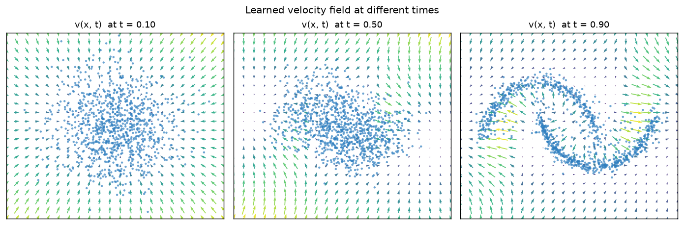
Early on the field points broadly inward, and by \(t \approx 0.9\) it resolves the target structure. See the Examples page to reproduce this.