Examples

The repository ships a runnable, tiered curriculum under examples/. Each example runs standalone in well under a minute on CPU, so you can read the source, run it, and tinker in one sitting.

Tier	Focus
00-foundations/	Core primitives in isolation (the linear interpolant)
10-sampling/	ODE sampling from a learned field (Euler flow)
20-training/	Flow-matching and delta-alignment training runs
30-inverse/	Posterior sampling for inverse problems
90-showcase/	End-to-end demos and visualizations

Run any of them the same way (from the repository root).

pip install -e ".[dev]"
python examples/00-foundations/01-linear-interpolant/main.py

---

00 foundations, the linear interpolant

examples/00-foundations/01-linear-interpolant/main.py

The interpolant is the smallest primitive in the whole library. It defines the probability path (how a noise sample and a data sample are blended at each time t) and, crucially, the target velocity the model is trained to predict. This example builds a LinearInterpolant, walks t from 0 to 1, and prints the intermediate point and its target velocity.

from deltaflow.interpolants import LinearInterpolant

interpolant = LinearInterpolant()
x1 = torch.randn(4, 2)   # data  (t=1)
x0 = torch.randn(4, 2)   # noise (t=0)

x_t, u_t = interpolant.interpolate(x1, t=torch.full((4,), 0.5), x0=x0)

What to notice.

• The path is the straight line \(x_t = (1-t)\,x_0 + t\,x_1\), so the target velocity is the constant displacement \(u_t = x_1 - x_0\). This is the delta the whole library is named after, the change that carries one distribution onto the other.
• The boundary conditions are exact. At t=0 the point equals x0, at t=1 it equals x1. The example asserts both, which is the sanity check every new interpolant must pass.

Run it first. Every later tier assumes you have this picture in your head.

---

10 sampling, Euler flow

examples/10-sampling/01-euler-flow/main.py

This is the shortest end-to-end story. Fit a tiny MLP velocity field on a two-Gaussian target with flow matching, then integrate it with FlowSampler (a thin Euler wrapper) to draw fresh samples.

field = MLPVelocityField(dim=2)
loss_fn = FlowMatchingLoss()
opt = torch.optim.Adam(field.parameters(), lr=2e-3)

for step in range(500):
    x1 = two_gaussians(256)
    loss = loss_fn(field, x1)         # samples x0, t internally
    opt.zero_grad(); loss.backward(); opt.step()

samples = FlowSampler(field).sample(torch.randn(1000, 2), n_steps=50)

What to notice.

• Training never runs the sampler. The loss draws its own x0 and t, so the loop is ordinary regression. Sampling is a separate, later step.
• FlowSampler.sample integrates \(dx/dt = v_\theta(x, t)\) with n_steps Euler updates. Fewer steps trade accuracy for speed, and straighter paths (see OT coupling) let you cut the count.
• The printed sample mean and std should land near the target's, a quick numerical check that the field learned the right transport.

---

20 training, flow matching in isolation

examples/20-training/01-flow-matching/main.py

The same objective as tier 10, stripped down to just the training loop on an anisotropic Gaussian. Use it as the reference for the loss signature and the loss_type option.

loss_fn = FlowMatchingLoss(loss_type="l2")
data = torch.randn(2000, 2) * torch.tensor([3.0, 1.0])

for step in range(300):
    x1 = data[torch.randint(len(data), (128,))]
    loss = loss_fn(field, x1)
    opt.zero_grad(); loss.backward(); opt.step()

See Flow Matching for the full objective and the interpolant options.

---

20 training, delta alignment

examples/20-training/02-delta-alignment/main.py

Delta alignment is the representation-learning half of the library. This example fits DeltaAlignmentLoss on synthetic multi-level feature maps, so you can see the API without wiring a full conditional backbone.

feature_dims = {"enc_1_4": 32, "enc_1_8": 64, "bottleneck": 128, "dec_1_8": 64}
projector = MultiScaleProjector(feature_dims, hidden_dim=64, out_dim=32)
loss_fn = DeltaAlignmentLoss(projector, lambda_flow=1.0, lambda_align=5.0)

total, loss_dict = loss_fn(
    v_c1, v_u1, target_v1,      # view 1: cond / uncond velocities + FM target
    v_c2, v_u2, target_v2,      # view 2
    feats_u1, feats_c1,         # view 1: per-level uncond / cond feature dicts
    feats_u2, feats_c2,         # view 2
)

What to notice.

• Two augmented views feed the loss. Each view carries a conditional and an unconditional feature dict at every hierarchy level.
• The loss aligns the guidance-difference feature (\Delta h = h_\text{cond}
• h_\text{uncond}) across the two views, not the raw features. The returned loss_dict breaks out each term for logging.

See Delta Alignment for the reasoning behind the difference feature.

---

20 training, conditional generation with a DiT

examples/20-training/03-conditional-dit/main.py

The native transformer path. A small DiT velocity field conditions on a class label through adaLN-Zero (Peebles & Xie, 2023), the shared time + class embedding drives per-block (shift, scale, gate) modulation, and the gates start at zero so the field begins as the identity. Two toy classes (bright-top versus bright-bottom 8x8 images) are learned with conditional flow matching, then sampled per class with classifier-free guidance.

from deltaflow.models import DiT

field = DiT(input_size=8, patch_size=2, in_channels=1, hidden_size=64,
            depth=2, num_heads=4, num_classes=2, class_dropout_prob=0.1)

loss = FlowMatchingLoss()(field, x1, y=y)   # label rides the opaque **cond channel

# guided sampling: extrapolate between the conditional and null-token velocity
v = field.forward_with_cfg(x, t, y=torch.zeros(64, dtype=torch.long), cfg_scale=2.0)

What to notice.

• The label enters through the same opaque **cond channel every DeltaFlow loss and solver forwards unchanged, here as y. No loss or solver needs to know about classes.
• LabelEmbedding carries a learned null token. Train-time label dropout teaches one network both the conditional and unconditional velocity, which is exactly what DiT.forward_with_cfg extrapolates between at sample time.
• The printed per-class pixel means separate cleanly (class 0 bright on top, class 1 bright on bottom), confirming the conditioning took effect.

---

30 inverse, posterior sampling

examples/30-inverse/01-posterior/main.py

The richest example. It trains a toy velocity field on synthetic Gaussian-blob images, samples unconditionally with EulerSolver, then reconstructs a centre-masked image with PosteriorSolver. It does this twice, once with OT coupling and once with independent coupling, mirroring the ablation that justifies OT as a default.

base = EulerSolver(model)
operator = MaskOperator(mask)
likelihood = GaussianLikelihood(y=y, operator=operator, sigma=1.0)

solver = PosteriorSolver(
    base_solver=base,
    likelihood=likelihood,
    tweedie=LinearTweedie(),
    guidance_scale=0.5,
    grad_normalize=True,
)
recon = solver.sample(torch.randn(n, 1, 16, 16), n_steps=50)

What to notice.

• PosteriorSolver wraps the same Euler solver used for unconditional sampling. It injects a measurement-likelihood gradient per step rather than re-implementing integration.
• The reported observed-region MSE lets you compare the two coupling strategies on the reconstruction task.
• The point is API wiring, not image quality. The dataset is synthetic and the backbone is deliberately tiny.

See Inverse Problems for the Tweedie step and the measurement operators.

---

90 showcase, sampling-flow visualization

examples/90-showcase/02-sampling-flow-viz/main.py trains a small MLP velocity field on a 2D two-moons target, records every intermediate sampling state, and produces four artifacts.

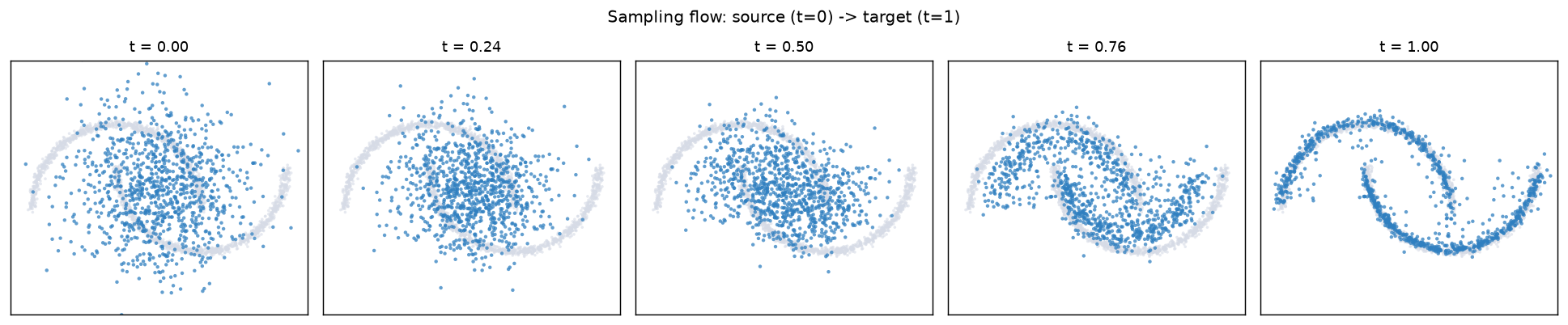
Source to target evolution. Noise (t=0) reshaped into the data manifold (t=1). The faint neutral cloud is the target reference.

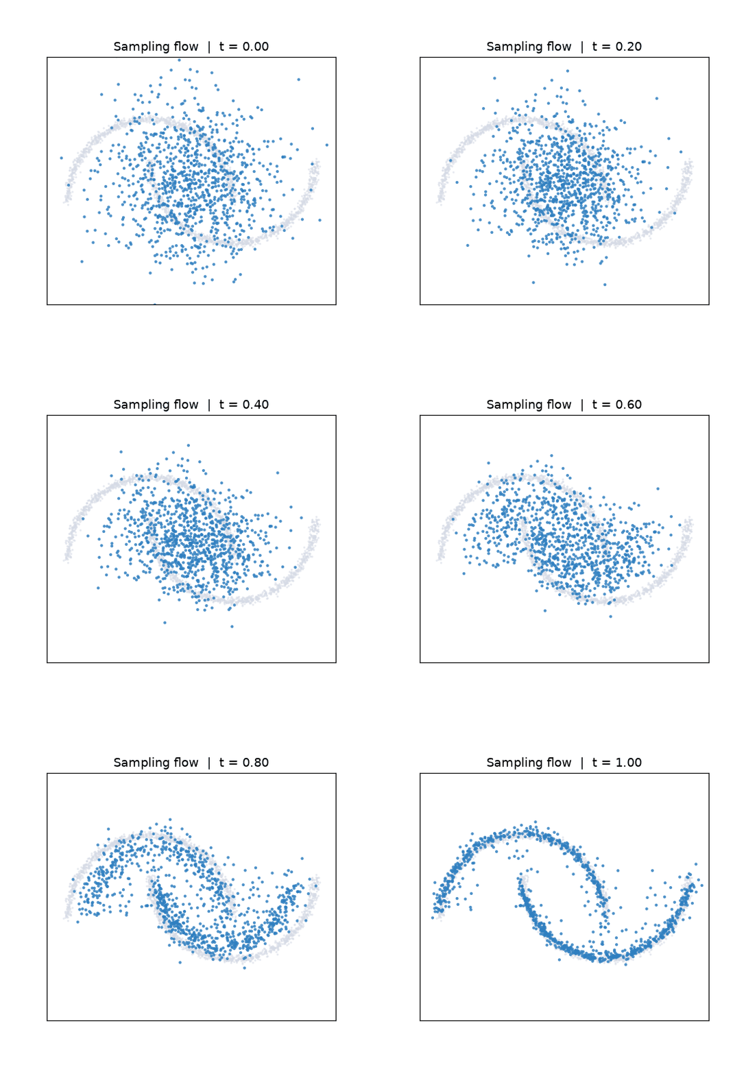
Animated sampling. The full Euler integration of the learned flow.

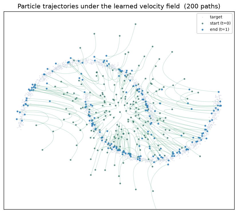
Particle trajectories. Individual paths from noise (deep teal, t=0) to data (teal, t=1), traced by green streamlines.

Learned velocity field. Quiver plots of \(v(x, t)\) at three times.

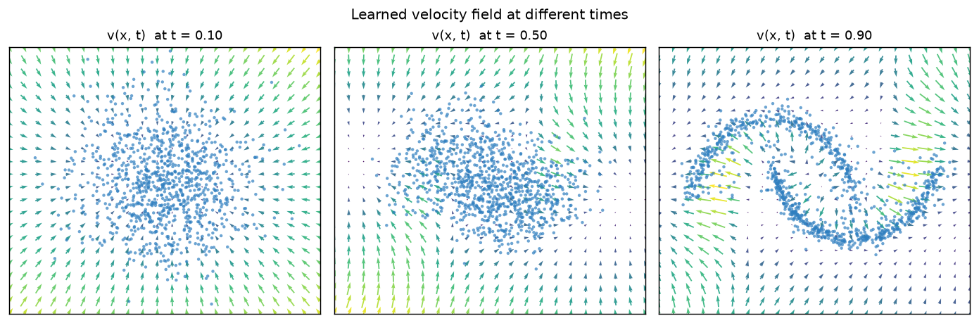
Early on the field points broadly inward. By \(t \approx 0.9\) it resolves the two-moons structure.

Reproduce

pip install -e ".[dev]" matplotlib
python examples/90-showcase/02-sampling-flow-viz/main.py
# artifacts are written to outputs/sampling_flow_viz/

90 showcase, mini-batch OT coupling

examples/90-showcase/03-minibatch-ot-viz/main.py contrasts two ways of pairing a source batch with a target batch before the flow-matching regression. The independent coupling pairs sample i with sample i, which scatters long crossing displacements across the batch. The mini-batch OT coupling solves a small assignment problem (squared-L2 cost) and reorders the target so each pair travels the shortest compatible distance.

Why it matters. Straighter pairings give the velocity field a smoother regression target, so trajectories bend less and few-step sampling stays accurate. The reported mean transport cost drops from the independent pairing to the OT pairing on the same points.

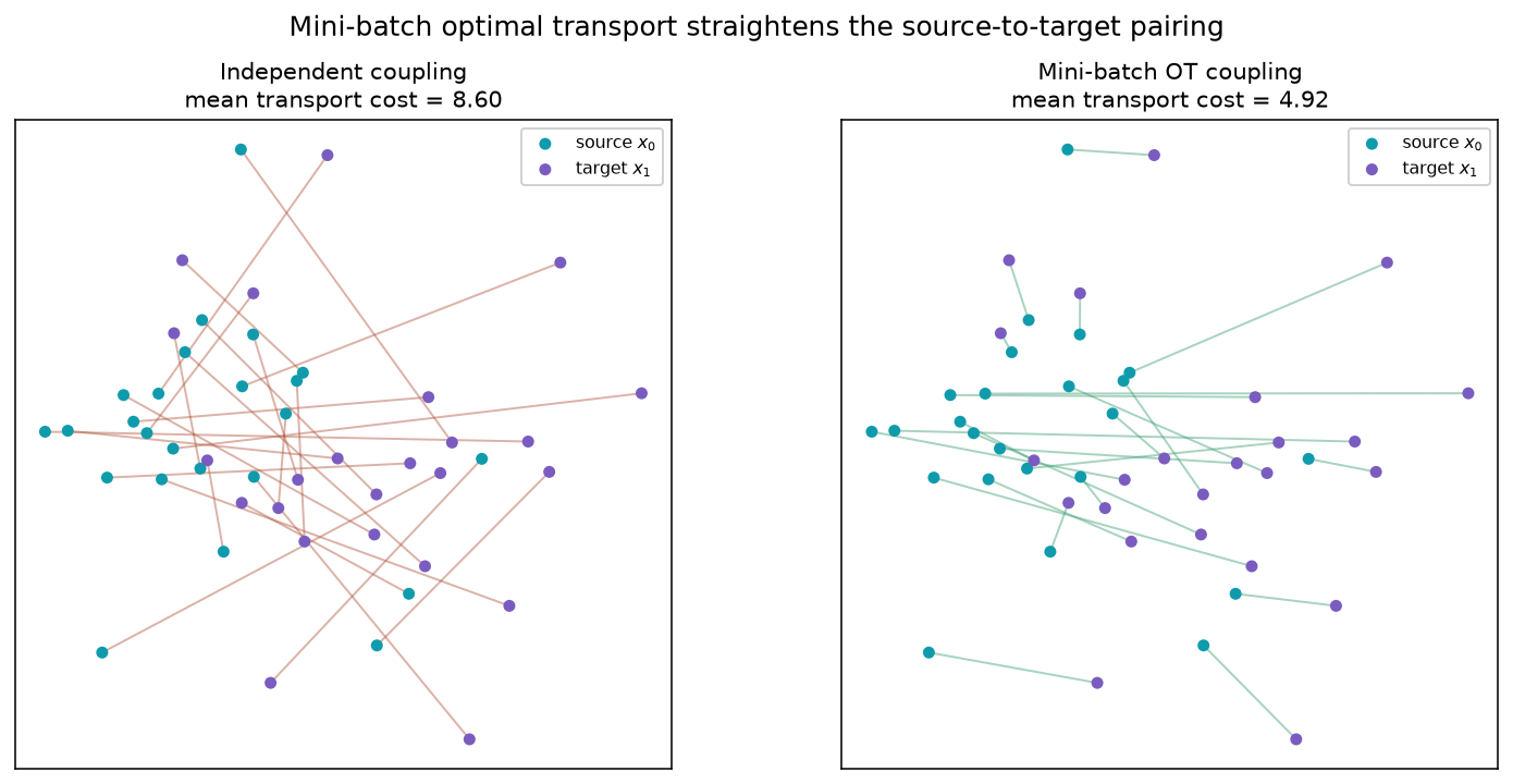
The source points are teal, the target points are purple. Notice how the tangle of crossings on the left collapses into a near-parallel bundle on the right.

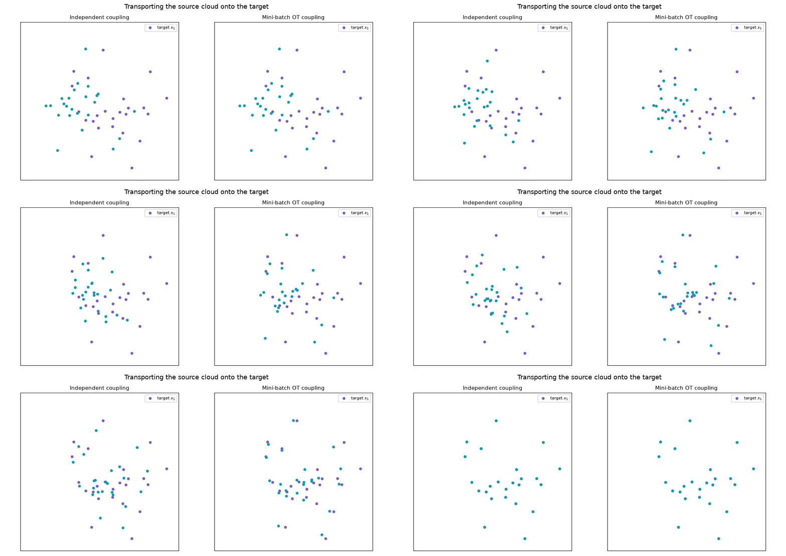
Animated transport. Both couplings carry the source cloud onto the same target. The OT bundle stays orderly while the independent pairing sweeps long crossing paths.

Reproduce

pip install -e ".[dev]" matplotlib
python examples/90-showcase/03-minibatch-ot-viz/main.py
# artifacts are written to outputs/minibatch_ot_viz/

90 showcase, inverse posterior sampling

examples/90-showcase/04-inverse-posterior-viz/main.py trains an unconditional flow on a small image family, then reconstructs a centre-masked measurement without any retraining. The PosteriorSolver steers the same learned flow with a measurement-likelihood gradient, so the known pixels stay fixed while the masked region is filled from the prior.

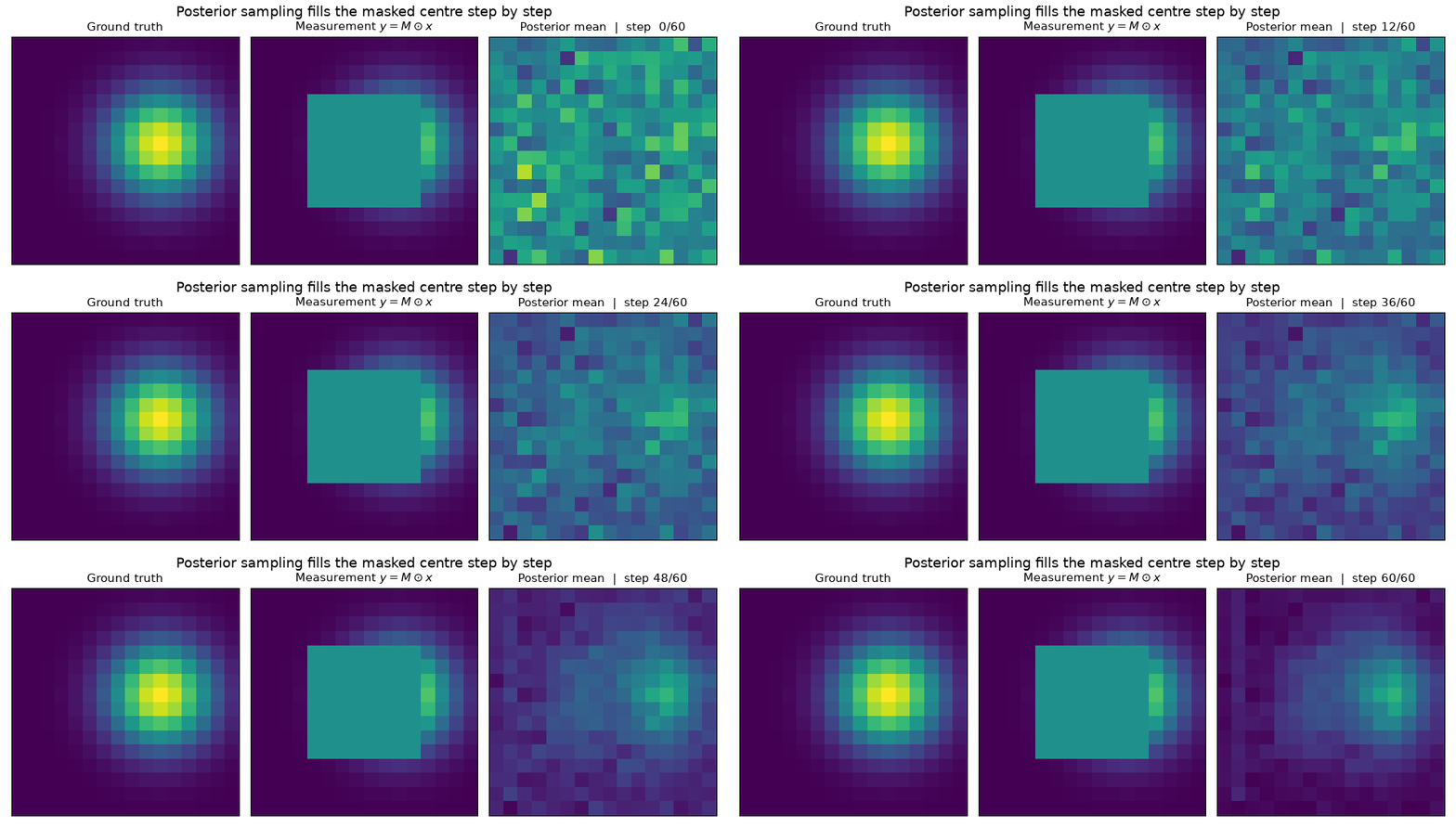
Why it matters. This is the inverse-problem workflow the library targets. One generative model, trained once, adapts to different measurement operators at sampling time. Here the operator is a binary centre mask, and the reconstruction is the mean over sixteen posterior samples.

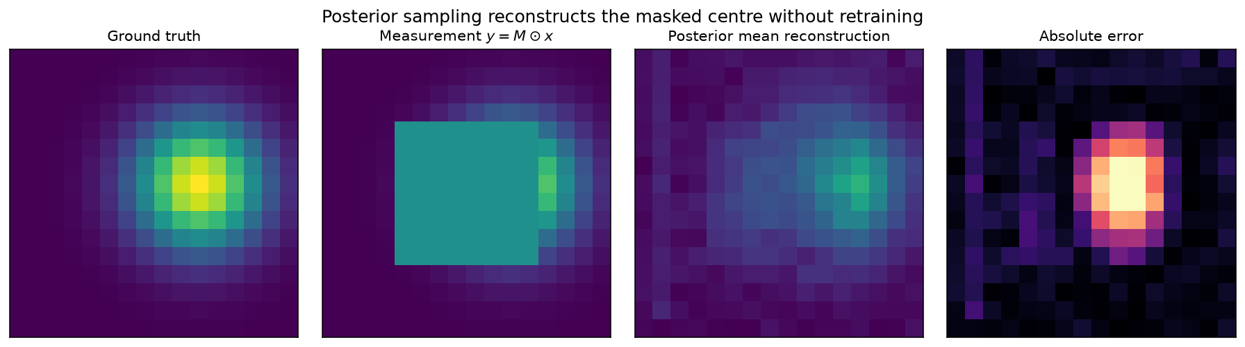
From left to right, the panels show the ground truth, the masked measurement, the posterior mean reconstruction, and the absolute error. The error concentrates inside the masked square, which is expected because the observed region is anchored by the likelihood.

Animated reconstruction. The posterior mean starts as noise and settles into the reconstruction as the solver walks from t=0 to t=1, guided at every step by the measurement likelihood.

Reproduce

pip install -e ".[dev]" matplotlib
python examples/90-showcase/04-inverse-posterior-viz/main.py
# artifacts are written to outputs/inverse_posterior_viz/

90 showcase, Schrödinger bridge

examples/90-showcase/05-schrodinger-bridge-viz/main.py first visualises the SchrodingerBridgeInterpolant path itself - the same (x0, x1) pair sampled repeatedly at increasing diffusivity sigma - then trains a velocity field against it (paired with OTCoupling) on a two-moons target and inspects the resulting sampler.

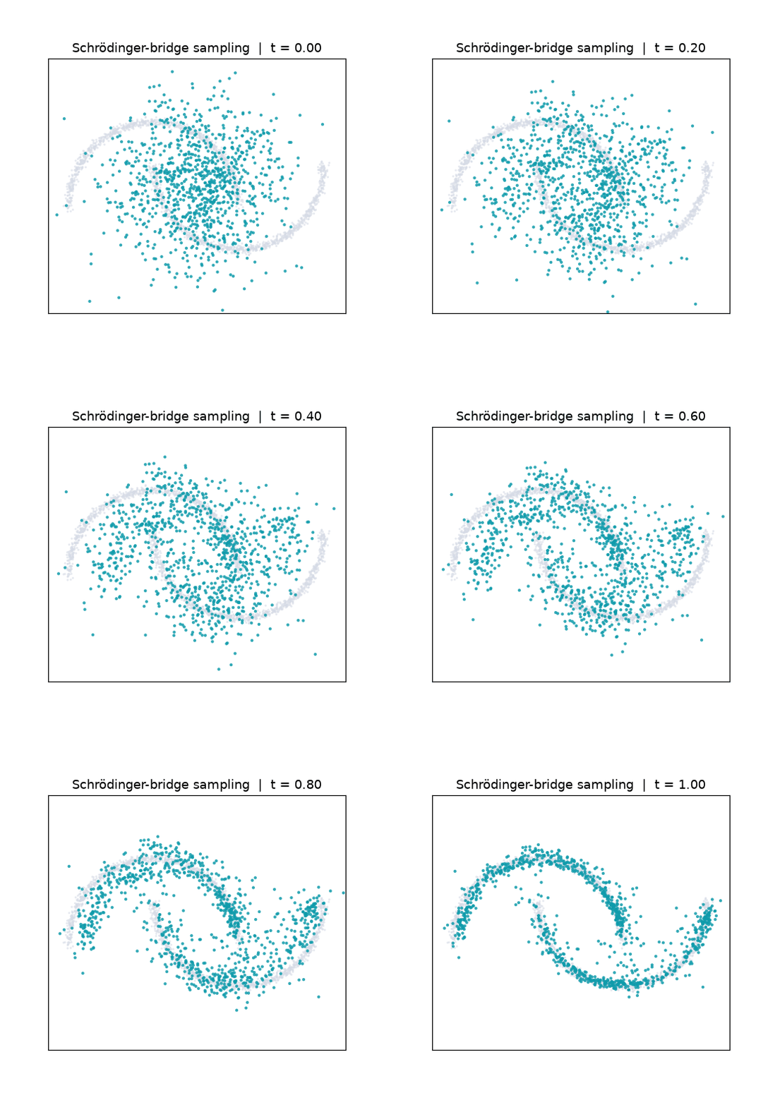
Why it matters. It is easy to conflate the stochastic training-time bridge with the learned sampler. Training regresses onto the conditional velocity of a noisy Brownian bridge, but generation integrates the resulting (deterministic) probability-flow ODE, exactly like the other flow-matching demos.

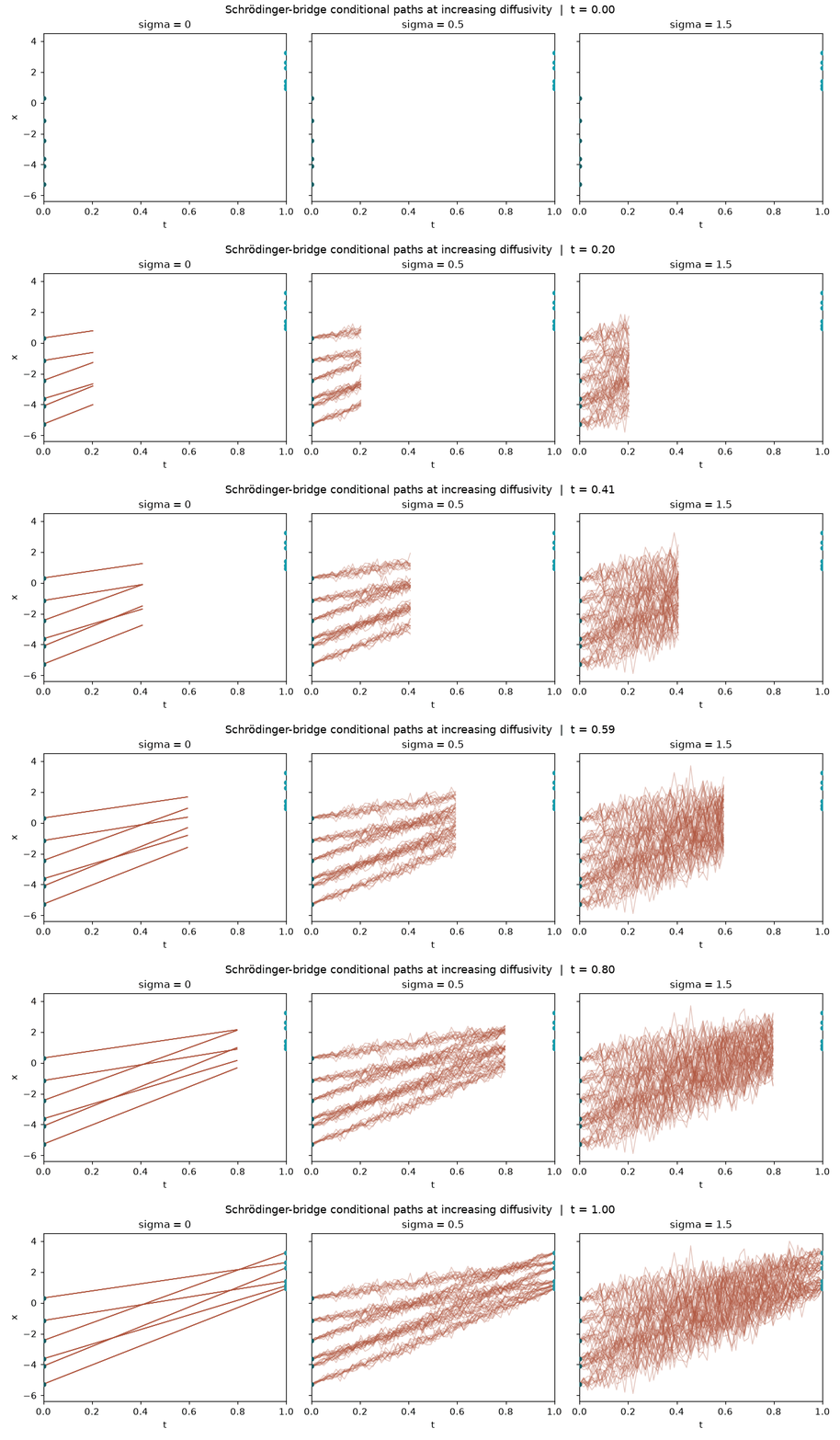
At sigma=0 the bridge collapses onto the straight line (LinearInterpolant exactly). Larger sigma widens the stochastic corridor the model must learn to regress against, without changing the deterministic ODE it produces.

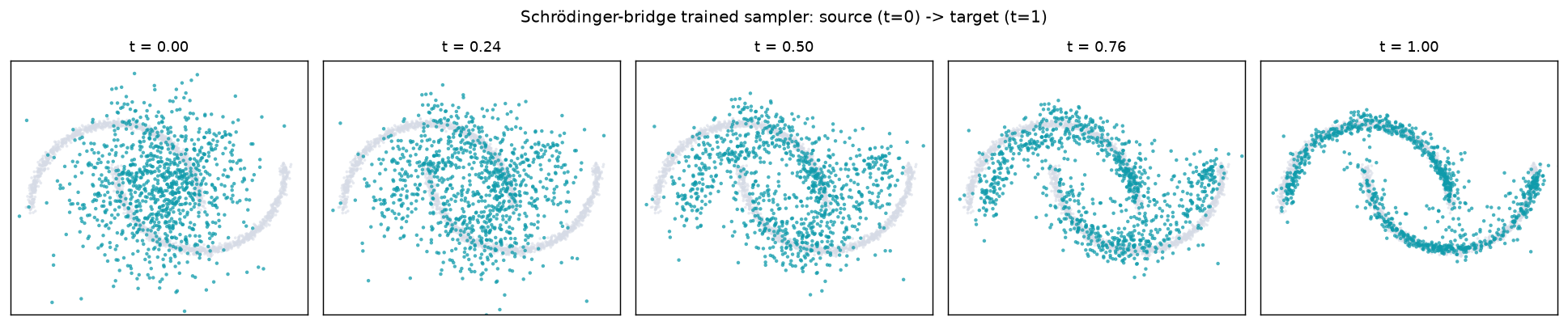
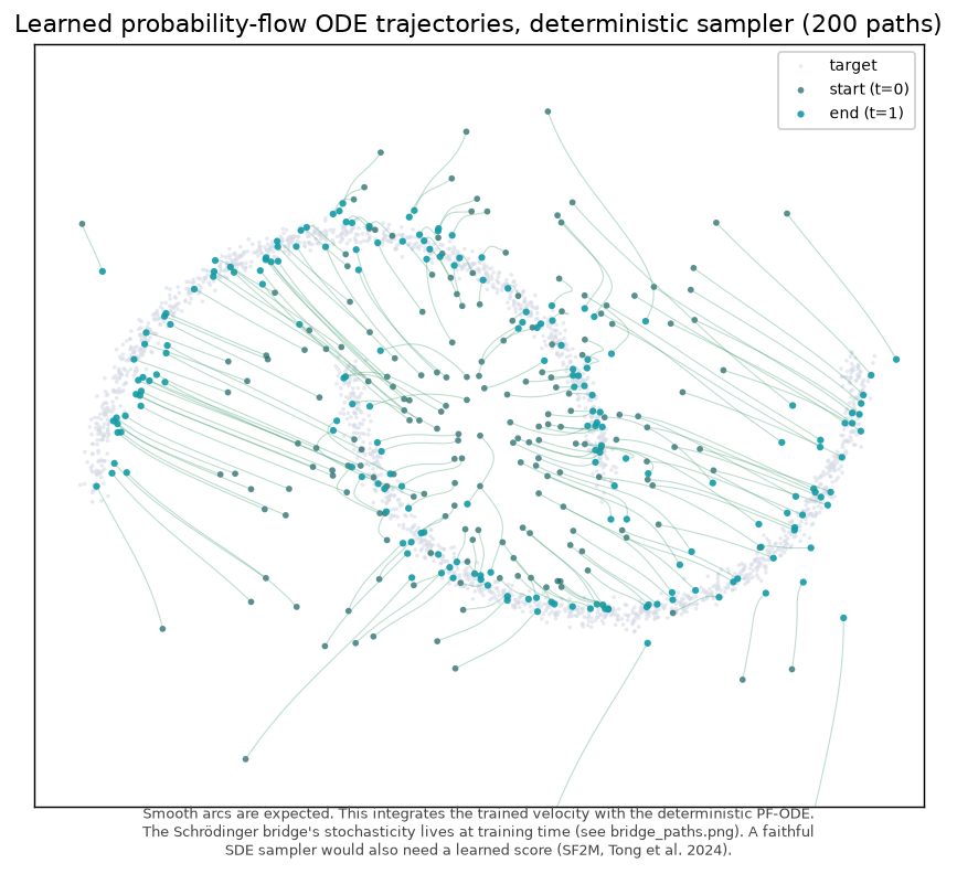
Animated sampling. The learned field integrates noise onto the two-moons target from t=0 to t=1, same as the flow-matching showcase, but the underlying field was trained on the bridge path above.

Reproduce

pip install -e ".[dev]" matplotlib
python examples/90-showcase/05-schrodinger-bridge-viz/main.py
# artifacts are written to outputs/schrodinger_bridge_viz/

90 showcase, comparing all four paths

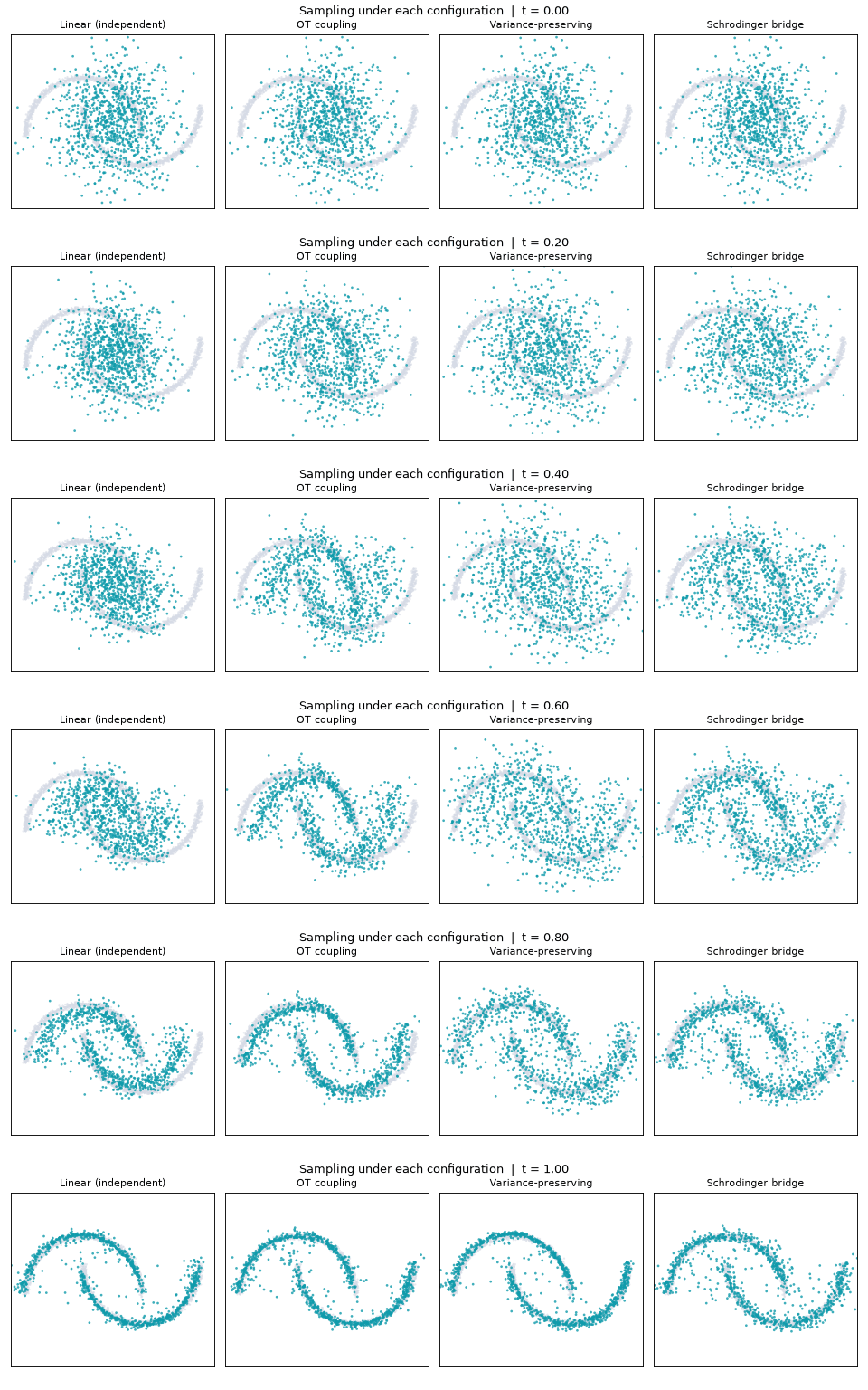
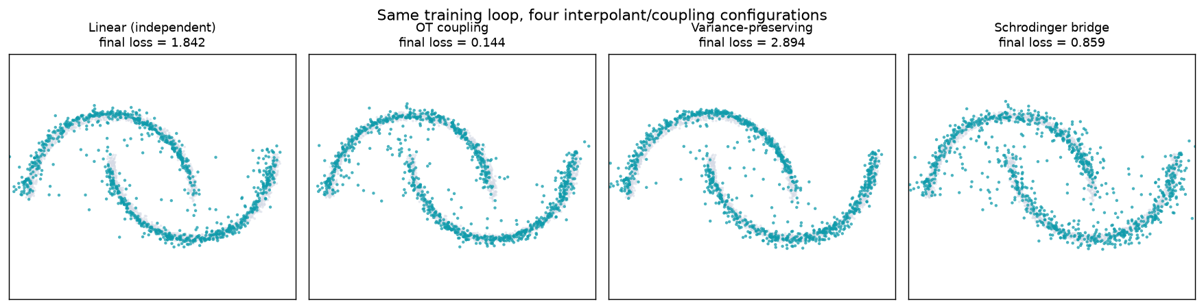
examples/90-showcase/06-algorithm-comparison/main.py trains the same MLP velocity field, for the same number of steps, on the same two-moons target, under four interpolant/coupling configurations, namely Linear with independent coupling, Linear with OTCoupling, VariancePreservingInterpolant, and SchrodingerBridgeInterpolant with OTCoupling.

Why it matters. Every DeltaFlow algorithm is a configuration of one training loop, and this demo makes the practical differences between configurations visible side by side, on identical data and compute budget.

Animated sampling, side by side. All four samplers integrate the same noise batch over the same number of steps, so the only variable on screen is the training configuration.

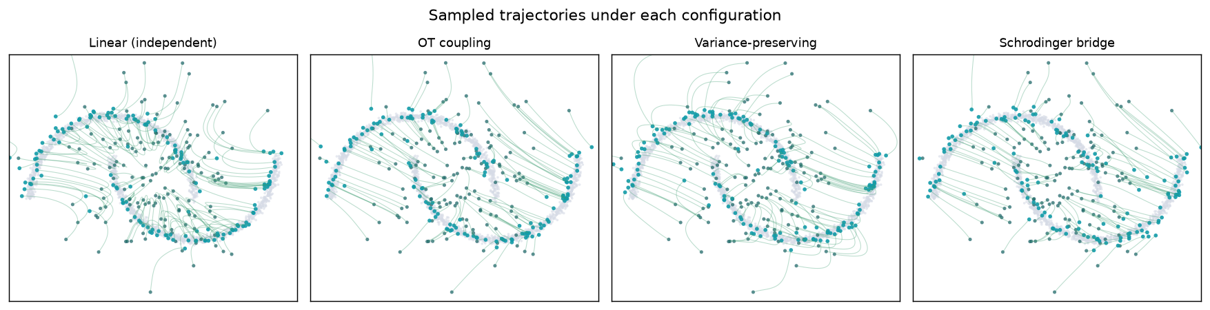
OT coupling produces visibly straighter trajectories than independent coupling, which is the point of minimising batch transport cost before regressing (see the 03-minibatch-ot-viz showcase above for why).

Reproduce

pip install -e ".[dev]" matplotlib
python examples/90-showcase/06-algorithm-comparison/main.py
# artifacts are written to outputs/algorithm_comparison/

90 showcase, landmark detection as conditional flow

examples/90-showcase/07-landmark-detection/main.py frames anatomical landmark detection as a conditional flow-matching problem, namely p(landmarks | image). The velocity field transports noise onto the stacked landmark coordinates while conditioning on the X-ray image, so sampling at inference time is detection.

Why it matters. It shows the discriminative use of a flow model, the image is the condition and the landmark coordinates are the generative target. This is the downstream counterpart to the representation-learning pretraining below.

The example runs on synthetic data by default and on the real ISBI2015 cephalometric set when pointed at it (both the per-image .txt layout and the Kaggle wide-CSV layout are auto-detected). It reports held-out flow-matching loss alongside mean pixel error.

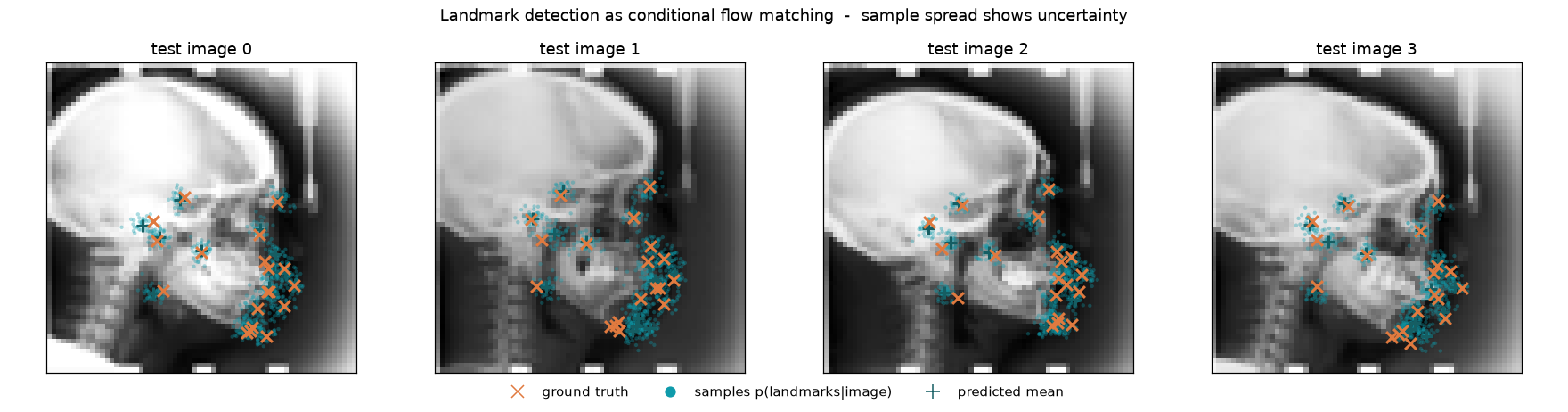
For each test image the model draws many samples from p(landmarks | image). The orange crosses are ground truth, the teal dots are posterior samples, and the teal plus marks are the per-landmark predicted mean. Tight sample clouds mean confident detections, wider spreads flag genuine positional uncertainty.

Reproduce

pip install -e ".[dev]" matplotlib
# synthetic default
python examples/90-showcase/07-landmark-detection/main.py
# real data (Kaggle ISBI2015 CSV layout)
python examples/90-showcase/07-landmark-detection/main.py \
    --data-root data/cephalometric/cepha400/cepha400 \
    --landmarks-root data/cephalometric/train_senior.csv \
    --test-landmarks-root data/cephalometric/test1_senior.csv \
    --n-landmarks 19 --image-size 64
# artifacts are written to outputs/landmark_detection/

90 showcase, guidance-aligned representation pretraining

examples/90-showcase/08-guidance-alignment-pretraining/main.py is the representation-learning half of the story, the CDPM-Align pretraining phase at toy scale. A small conditional UNet velocity field learns p(image | y), where y is a dataset/class label (not a landmark), with a learned null class for classifier-free guidance. At every hierarchy level the guidance difference delta_h = h_cond - h_uncond is projected by a MultiScaleProjector and aligned across two noise-level views with DeltaAlignmentLoss (the "Delta" in DeltaFlow).

Why it matters. It answers "condition on the image or on the landmark?". Pretraining conditions on the image and generates the image, landmarks are never used here. The claim is that guided generative pretraining yields an anatomy-discriminative representation. We check this by freezing the backbone and fitting a linear probe on its features, comparing against a random-init backbone.

On the synthetic four-dataset task the probe reaches near-perfect accuracy on held-out images (chance is 0.25) while the random-init baseline sits far lower, and a PCA of the frozen features separates cleanly by dataset. The alignment term is a light consistency regularizer on delta_h and stays small on this easy task, its role grows on harder heterogeneous data.

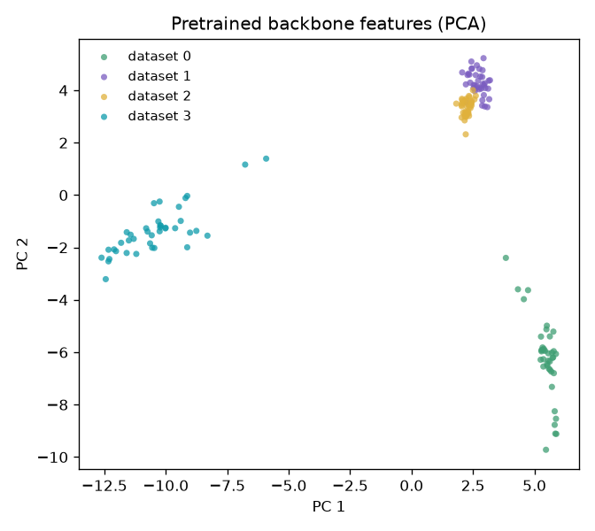
Each dot is a held-out image placed by its frozen bottleneck feature, reduced to 2D with PCA. Tight, well-separated colours mean the representation encodes dataset/anatomy identity, which is why the linear probe is trivially accurate. A random-init backbone would show the colours largely mixed.

Reproduce

pip install -e ".[dev]" matplotlib
python examples/90-showcase/08-guidance-alignment-pretraining/main.py
# artifacts are written to outputs/guidance_alignment_pretraining/

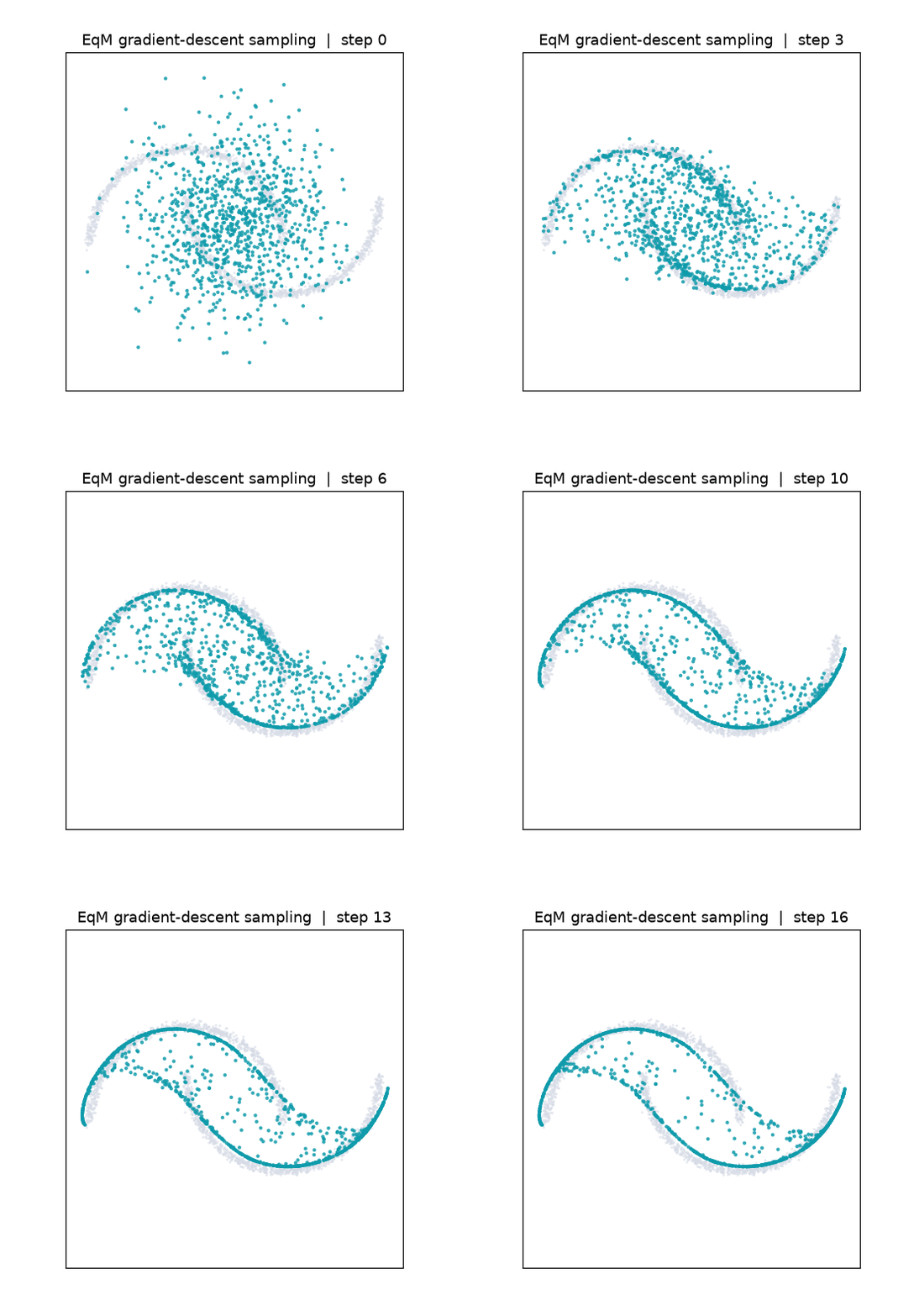
90 showcase, Equilibrium Matching landscape and sampling

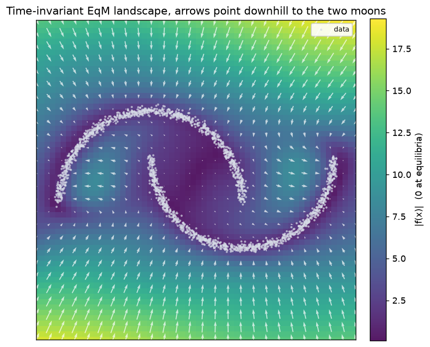
examples/90-showcase/09-equilibrium-matching-viz/main.py trains a noise-unconditional field with EquilibriumMatchingLoss on the same 2D two-moons target as the flow-matching showcase above, then samples it by gradient descent on the learned landscape (no ODE integration). Reusing the dataset makes the contrast with flow matching direct. Equilibrium Matching drops the time-conditional dynamics of flow models, so the field \(f(x)\) is time-invariant and a single picture of it describes the whole sampler. The interpolation coefficient \(\gamma\) is implicit and never seen by the model.

Time-invariant landscape. Arrows are the field \(f(x)\), the heatmap is the gradient norm \(|f(x)|\). The norm collapses toward zero along the two moons, so those points are the equilibria (minima) of the implicit energy the field descends. One panel replaces the per-time quiver the flow-matching showcase needs.

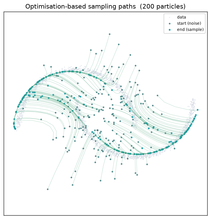
Gradient-descent sampling. Pure noise settles onto the two moons as the optimisation-based sampler iterates. Compare the final panel with the flow-matching snapshots above, both recover the same target by very different mechanics (gradient descent on a static landscape versus ODE integration of a time-varying velocity).

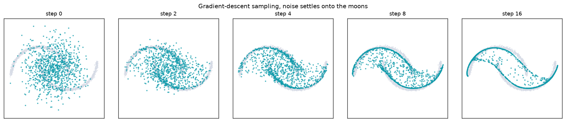
Animated sampling. The full gradient-descent run.

Particle trajectories. Individual paths from noise (deep teal) to the samples (teal), traced by green streamlines.

Reproduce

pip install -e ".[dev]" matplotlib
python examples/90-showcase/09-equilibrium-matching-viz/main.py
# artifacts are written to outputs/equilibrium_matching_viz/