DeltaFlow

DeltaFlow provides composable PyTorch primitives for generative modelling in data-scarce domains such as medical imaging, with a focus on representation learning and studying the underlying data distribution (not just sample synthesis).

• Getting Started

  Install DeltaFlow and fit your first flow-matching model in a few lines.

• Guides

  Task-oriented walkthroughs covering flow matching, delta alignment, training, and inverse problems.

• Architecture

  The four base abstractions that make every component drop-in.

• API Reference

  Auto-generated documentation for every public class and function.

What is DeltaFlow?

DeltaFlow is built on a single idea, a delta (the change carried from one distribution to another) and the flow that realises it.

• Δ, the change between two things. The learning signal is a displacement \(\Delta = x_1 - x_0\), the straight-line velocity carrying a source sample \(x_0\) (noise) to a data sample \(x_1\). Regressing a velocity field onto \(\Delta\) is exactly the flow-matching objective (Lipman et al., 2023).
• Flow, integrating the change. A learned field \(v_\theta(x, t)\) is integrated as an ODE \(dx/dt = v_\theta(x, t)\), transporting the whole source distribution onto the data distribution.
• Straighter Δ via optimal transport. Mini-batch optimal-transport coupling solves the discrete Kantorovich assignment on each batch, the source to target pairing that minimises squared transport cost, so the displacements, and the flow that follows them, are as straight as possible and sample in fewer steps. This hard assignment is the zero-entropy limit of the static Schrödinger bridge (Tong et al., 2023).

The same difference principle also drives an optional representation-learning loss, delta alignment, which aligns the guidance-difference feature \(\Delta h = h_\text{cond} - h_\text{uncond}\) for generative pretraining in data-scarce domains.

The library targets 2D radiography (chest X-ray, cephalometric, and hand radiographs), but the core primitives (interpolants, samplers, losses, models.projector) are domain-agnostic.

Visualizing the algorithm

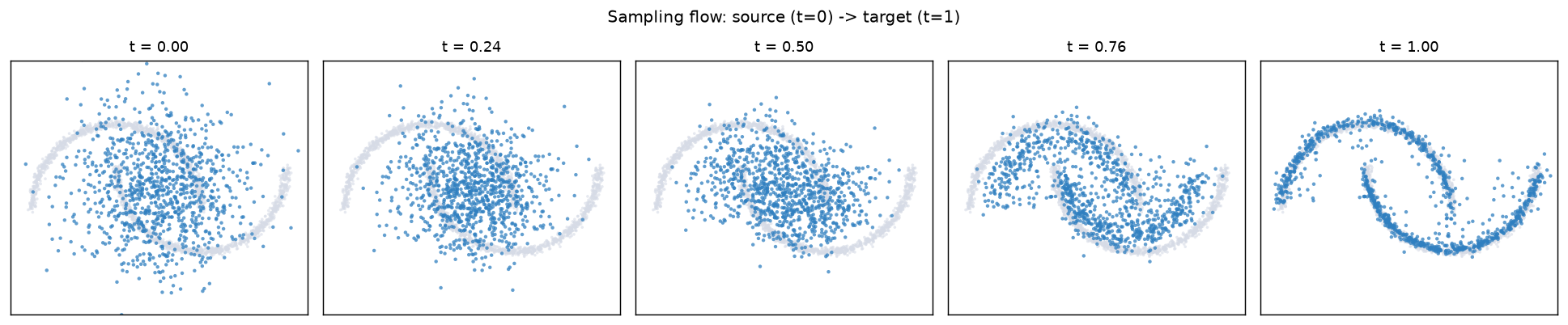
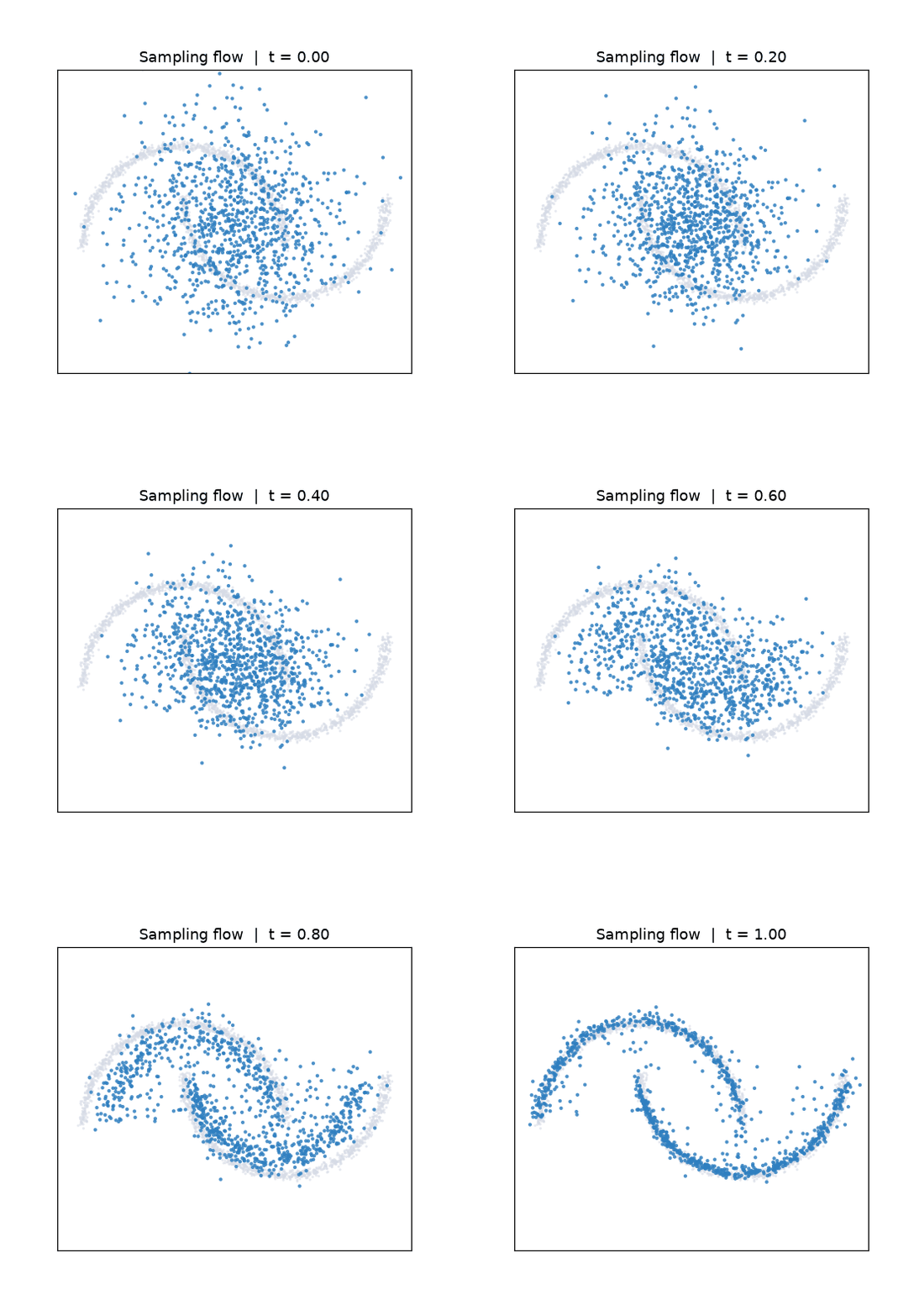
Flow matching learns a time-conditioned velocity field \(v(x, t)\) that transports a simple source density (Gaussian noise, \(t=0\)) onto the data distribution (\(t=1\)). The panels below come from the sampling-flow example.

Probability paths

The interpolant= argument selects the path noise and data connect along. The same training loop, loss, and solver are reused across all of them.

Interpolant	Path
LinearInterpolant	straight-line rectified-flow path, \(x_t = (1-t)x_0 + t x_1\)
VariancePreservingInterpolant	trigonometric diffusion path, \(\alpha_t = \sin(\tfrac{\pi}{2}t)\), \(\sigma_t = \cos(\tfrac{\pi}{2}t)\)
OTInterpolant	the linear path applied after a mini-batch OT re-ordering of \(x_0\)
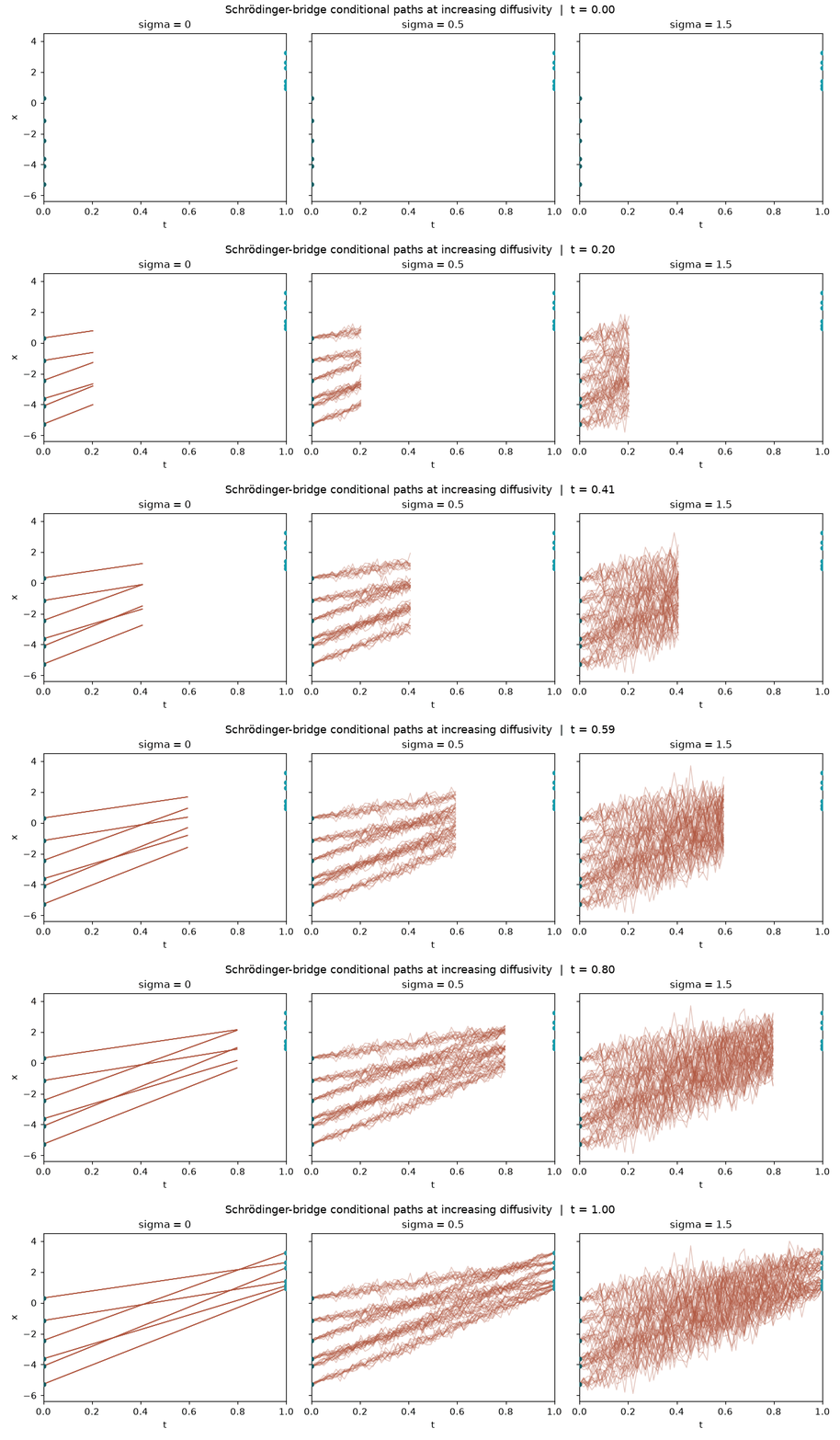
SchrodingerBridgeInterpolant	entropic Schrödinger-bridge path, a Brownian bridge \(x_t = (1-t)x_0 + t x_1 + \sigma\sqrt{t(1-t)}\,z\) around the straight line, diffusivity \(\sigma\)

Schrödinger bridge

The dynamic Schrödinger bridge between noise and data, conditioned on an endpoint pair, is a Brownian bridge around the straight-line path. Regressing onto its conditional velocity trains a stochastic interpolant that recovers the entropic optimal-transport bridge as the coupling of \((x_0, x_1)\) approaches the true OT plan. Pairing endpoints with OTCoupling (rather than drawing them independently) is what makes this approximation tight in practice (De Bortoli et al., 2021 and SF2M, Tong et al., 2024).

Comparing the paths

Every algorithm is the same training loop. Only the interpolant= (and optionally coupling=) argument changes. Training an identical MLP on a two-moons target with each configuration for the same number of steps makes the differences concrete. All four samplers below are integrated from the same noise batch at the same number of steps.

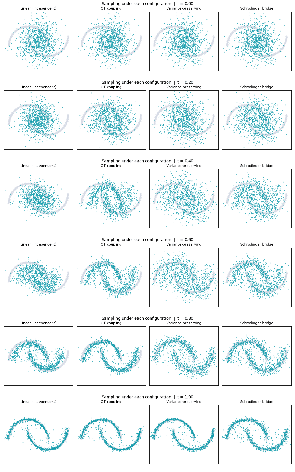
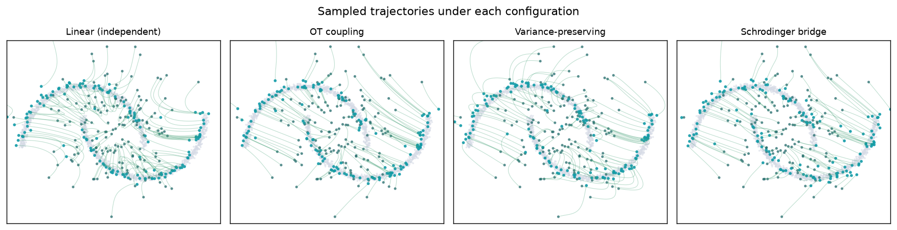
OT coupling produces the straightest source-to-target trajectories of the four, the practical benefit of minimising batch transport cost before regressing. Reproduce these figures from the algorithm-comparison showcase.

What's inside

Module	Role
deltaflow.core	Abstract base classes every component subclasses
deltaflow.interpolants	Probability paths (linear, mini-batch OT, variance-preserving, Schrödinger bridge)
deltaflow.samplers / deltaflow.solvers	Euler & Heun integration, posterior sampling
deltaflow.losses	Flow matching + delta alignment
deltaflow.models	Backbones, EMA, multi-scale projector heads
deltaflow.inverse	Measurement operators, Tweedie decomposition, likelihoods
deltaflow.trainer	Streaming data, mixed-precision loop, OT coupling
deltaflow.datasets	Radiograph dataset wrappers (chest / cephalo / hand)

Citation

If you use DeltaFlow in your research, please cite it (see CITATION.cff).